Undetermined Coefficient

The Undetermined Coefficient is one of the ways to find the particular solution to a non-homogeneous differential equation.

The advantage with this approach is reduces the problem to an algebra problem. However, this may work only on limited classes of g(t).

We can write y(x) as,

 Where,

Let's solve this given SODE,

 We first solve for yh,

 Since they are real roots, we have yh as,

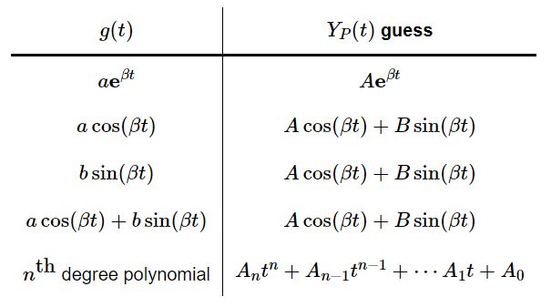
For yp, we have to guess what it looks like based on g(x). The table below will help us to determine that.

Since g(x) = 3e^(5x), then our yp guess is,

We can plug yp guess to get our actual yp,

we now have y(x) and y'(x) as follows,

To get c1 and c2, we set x = 0 with the above equations,

Now, we have our actual solution,

Separable First-Order of Differential Equation

A first-order differential equation is said to be separable if , after solving for the the derivative,

 the right-hand side can be factored by function of x and function of y,

If the factoring is not possible, this means that the derivative is not separable.

Let's have an example,

First, we check if it is separable,

Since it is separable, we can continue solving it by integrating both sides:

Another application for this is with Lotka-Voltera model of predator y - prey x dynamics.
It is given by,

 Where,

 Independently, they can't be solve in linear method. However, the dependence of the predator prey population can be solve by,

 This now becomes a separable fode as proof below,

After we integrate both sides, we are left with an implicit function.

Fourier Series Approximation

Fourier Transformation is a function f(t) derived from a given function and representing it by a series of sinusoidal functions. It is expressed as:

where,

It is used in multiple fields like signal and noise estimation, seismographs, and filtering.

To show how it works, we'll give the Fourier series of the given functions:

Since both of these functions is at t(0), we need to shift the charging formula.

If plotted, it will result to this:

Note that which equation Q(t) to use depends on time t,

To solve a0,

To solve an,

To solve bn,

By plugging the values, we will have f(t) as,

As we increase the approximation term n , the series approximation improves as well.

LU Factorization

LU Factorization is used to factor matrix A as the product of lower-triangular matrix L and upper-triangular matrix U.

A = LU

In order to do such decomposition, one must have the knowledge of Gaussian Elimination. 

To better understand how this works, given the matrix M below, we'll get it's LU Decomposition.

To get U we will do the following transformation: 

A lot of us (or maybe just me) have at least once imagined what it be like to become spy. With their high-tech gadgets, jaw-dropping acrobatic stunts, and, more importantly, a covert life. We often see in movies that they pass around unreadable messages that seems to make no sense. But we eventually see that every message is just puzzle that is yet to be decoded.

Let's have an activity where we will try to decode this message:

The given encoded message was derived from this equation:

In order to get the original message (M),  we can rewrite the equation to:

And we already have an agreement with the sender that our encoding matrix will be:

We need to first solve for the inverse of C. This can be done via LU Decomposition.

Now, it is just a matter of plugging in our values:

The result is represented by their ASCII values, so we can convert each of them.

And we will have the original message,

"Sherman - Morrison Formula!"

Which is actually the name of the formula we used to encode our message!